Decoding the Decisions
Introduction
Across every sport, fans will boo referees when a call doesn’t go their way. They emphatically explain how they’re being paid off and rigging it in real time. Basketball is no exception. And indeed, there may have been cases of referees interfering and throwing a game, but how large of an effect are they really having on a daily basis?
To answer this, I pored through a database of over 64,000 NBA games that includes box scores, play-by-play data, and a most importantly, a list of referees for each game. I preprocessed the SQL database of games so that I had the two teams playing, their scores, and the three referees for the game, and was ready to dive in.
Method 1: Points added from referee
The most basic way of seeing how much a particular referee impacts a team is by calculating the average score of the team over the dataset (in this particular case, starting in the 1996 NBA season – referee data isn’t included before then), and then comparing that the to average score of the team when a particular referee officiates the game. This is easy to do in Python by connecting to the SQL database with the sqlite3 library then creating a dataframe in pandas.
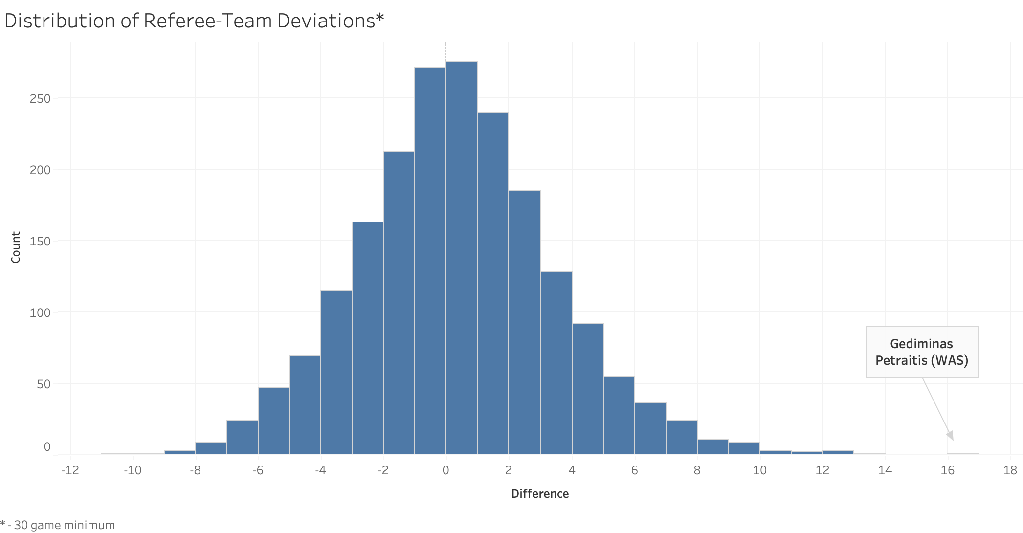
After conducting exploratory analysis on the dataframe, a new table was generated showing the specific referee and NBA team combinations along with the differential compared to how that team normally performs. To ensure the analysis includes only referees who have officiated a substantial number of games for a given team, a threshold of a minimum of 30 games officiated per team was set. Presented below are the top ten referee-team pairings ranked by the absolute value of the difference in average scores.
A few things stand out in this top ten. Nine of ten of the entries are positive, indicating that the referee gave the particular team an advantage, while only one (when Kevin Fehr officiates the Clippers) creates a disadvantage. Does this mean that referees are more interested in helping certain teams than hurting others? There are multiple repeated referee names among the top results, including Gediminias Petraitas, Tyler Ford, and Mitchell Ervin, each appearing twice. These deviations are quite large — all double digits. Is Gediminas Petraitis really having a sixteen point difference on games?
To further investigate this discrepancy, the data was visualized by overlaying all Wizard’s games, including those officiated by Gediminias Petraitas, in Tableau. This visualization highlighted that the dataset is incomplete for certain years, most notably 2018, emphasizing the importance of comprehensive data coverage for robust analysis. In the visualization, each solid black dot denotes a game officiated by Petraitas.
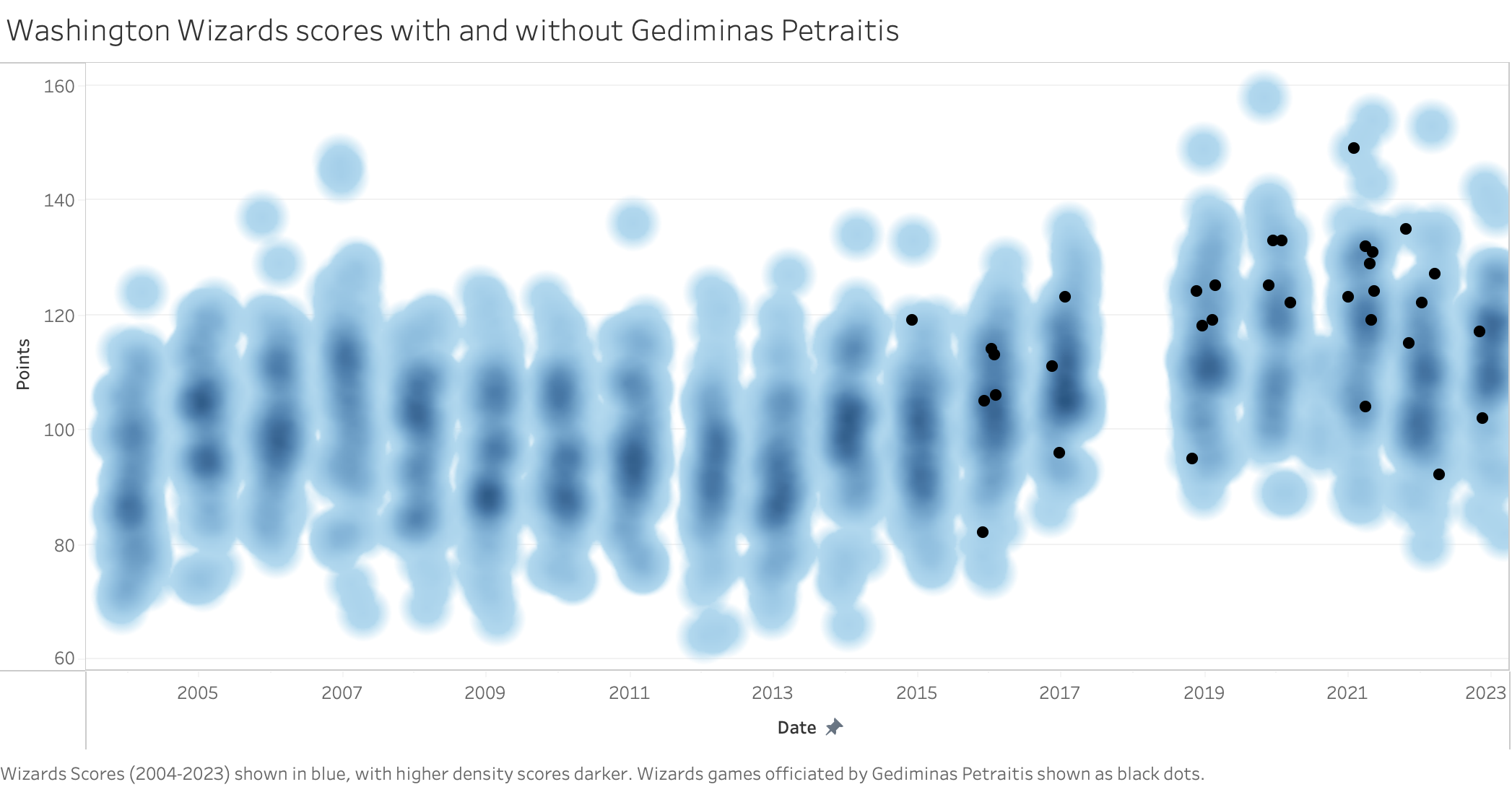
This visualization tells a much different story. Instead of Petraitas consistently adding double digits above the Wizards’ expected score, he happened to officiate games when the Wizard’s had their highest scoring seasons. Indeed, this is not just a Wizards phenomenon, but a league-wide one. The Wizards average points per game (PPG) in the 2014-2015 season was 98.5, 17th in the league, and increased to 114.4 PPG in the 2019-2020 season, a very significant increase, placing 7th in the league by PPG. Over the same period, the NBA league average increased from 100.0 to 111.8, likely due to more emphasis on three pointers and increasingly faster paced games.
Method 2: Elo System
Rather than calculating the average over the full dataset, an “Elo” rating system was implemented whereby referees would receive greater penalties for larger deviations from a team’s expected average score in a given time period. Specifically, for each game the score with a particular referee was subtracted from the team’s average that season rather than the overall average across all seasons.
In the previous example with Petraitas, instead of the Wizard’s 146-149 loss on 1/31/21 counting as a 47 point deviation, it is roughly 31 points.
This analysis paints a much less extreme picture. Presented below are the top ten referee-team pairings using this revised metric:
In this ranking, none of the referee-team combinations exceed double digit point differences. Indeed, the margins approach approximately 5 points very rapidly. Notably, the previously analyzed Petraitis pairing ranks second. Mark Ayotte, with 49 New York Knicks games officiated within the dataset, shows an average benefit of nearly 7.5 points for that team. As with the prior analysis, the data was visualized in Tableau to assess whether the deviation appears extreme.
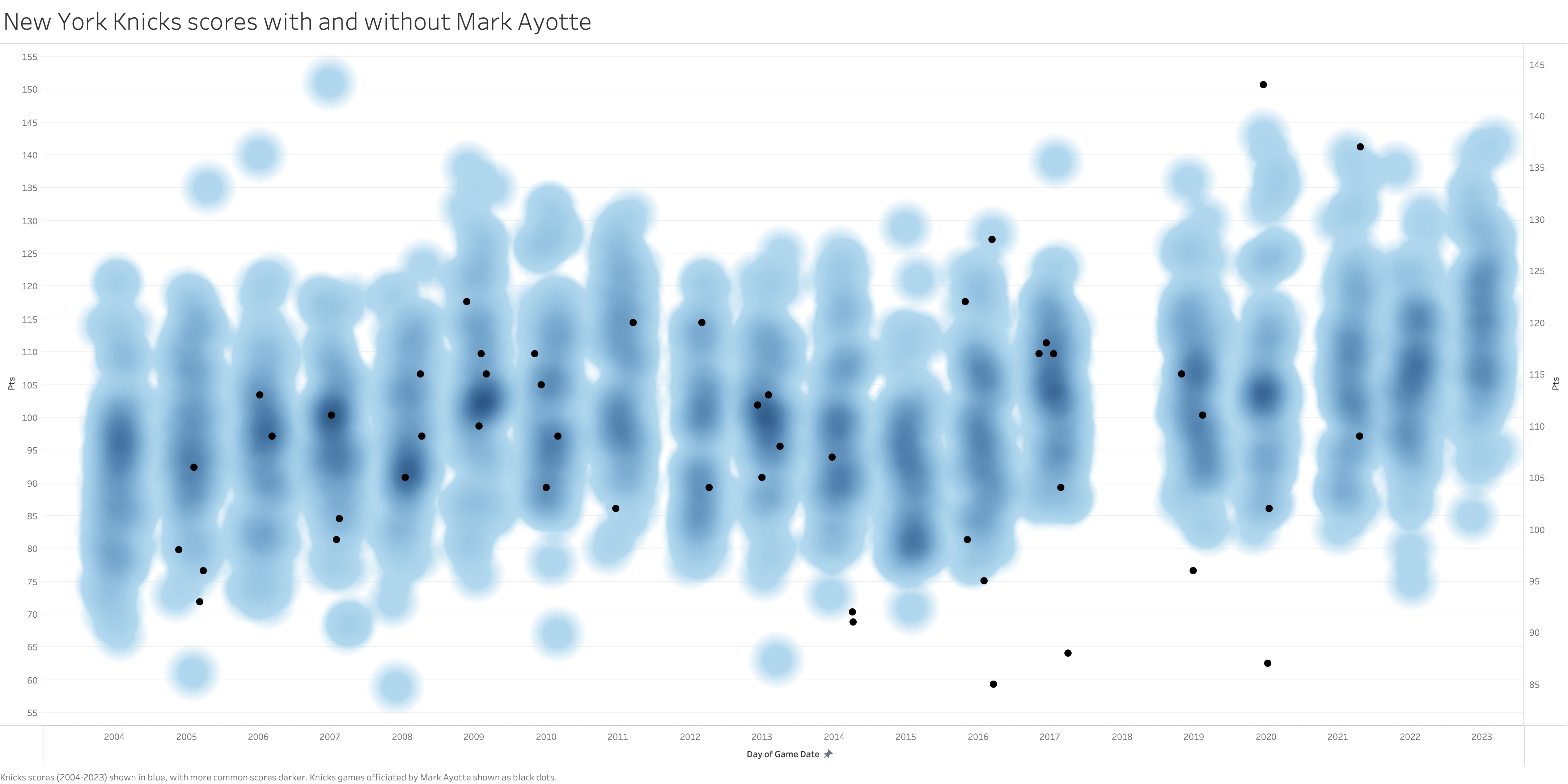
Similarly, there seems to be no clear pattern of Mark Ayotte helping the Knicks score more points even though the data suggests it. In fact, there were a few games between 2014-2017 where NYK games officiated by Ayotte are near the bottom of their season scoring. However, the outlier games (143 points against the Hawks in 2019 and 137 points also against the Hawks in 2021) more than offset these.
So far, no convincing evidence has been found to suggest that referees in the league systematically favor or disadvantage specific teams. It should be noted that this analysis does not account for high-stakes playoff games or isolated incidents, which require individual examination. A major call occurring with five seconds remaining that results in two points is statistically equivalent to a shooting foul committed two minutes into the first quarter.
Method 3: Impact Score
The focus has initially been on points, using only subtraction of means for the analysis. However, this study can be broadened to include all metrics provided in the original database for each team in a given game: field goals made, field goal percentage, three pointers made, three point percentage, free throws made, free throw percentage, offensive rebounds, defensive rebounds, total rebounds, assists, steals, blocks, turnovers, and personal fouls. This offers a wider range of data for analysis, but introduces the challenge of working with multiple dimensions simultaneously.
The objective is to reduce the dataset’s number of dimensions to a more manageable size, ideally one or two, without losing significant information. One effective method for achieving this is principal component analysis (PCA). PCA employs linear algebra to identify the principal components of the dataset. The first principal component accounts for the most variance in the data. Subsequent components, each orthogonal to the preceding ones, account for decreasing amounts of variance. As a result of this orthogonality, each principal component is uncorrelated with the others.
For implementation, some pre-processing is necessary. The original SQLite database was modified so that each row now represents the performance of a single team in a game across all listed metrics, as well as one of the referees involved. Consequently, six rows are present for each game that involves three referees.
Following these modifications, the means of each statistic for every referee were calculated and aggregated into a new table:
# List of columns that contain statistics
stats_columns = ['fgm', 'fg_pct', 'fg3m', 'fg3_pct', 'ftm', 'ft_pct', 'oreb', 'dreb', 'reb', 'ast', 'stl', 'blk', 'tov', 'pf', 'pts']

# Group by referee and aggregate the original data
aggregated_raw_data = data.groupby(['first_name', 'last_name', 'official_id']).agg({**{col: 'mean' for col in stats_columns}, 'game_date': 'count'}).reset_index()
aggregated_raw_data = aggregated_raw_data.rename(columns={'game_date': 'num_games'})
Before proceeding to PCA in R, it is essential to normalize the data. This ensures that statistics with higher means, such as points, do not disproportionately influence the analysis. The mean and standard deviation for each statistic will be calculated. Subsequently, these values will be used to standardize each official’s statistics by subtracting the mean and dividing by the standard deviation. This standardization process results in a mean of zero and a standard deviation of one for every statistic:
# Normalize the aggregated data
aggregated_raw_data[stats_columns] = (aggregated_raw_data[stats_columns] - aggregated_raw_data[stats_columns].mean()) / aggregated_raw_data[stats_columns].std()
Now our data is ready for principal component analysis. We’ll export this dataframe to R:
# Perform PCA
pca_result <- prcomp(data_pca_only, scale. = TRUE, center = TRUE)

# Extract the scores for each principal component
scores <- pca_result$x

# Append the PC scores to the original dataframe
data_with_scores <- cbind(data_for_pca, scores)
Two parameters for prcomp, scale. = TRUE and center = TRUE, indicate that standardization is performed internally, making prior normalization optional. However, standardizing the original dataframe provides flexibility for potential use in other contexts where automatic standardization is not available. To interpret the principal components, attention is first given to the relative weights or loadings assigned to each variable by running print(pca_result$rotation).
| PC1 | PC2 | PC3 | PC4 | PC5 | PC6 | PC7 | PC8 | PC9 | |
|---|---|---|---|---|---|---|---|---|---|
| fgm | -0.315 | 0.040 | -0.031 | 0.084 | 0.067 | 0.038 | 0.025 | -0.118 | -0.202 |
| fg_pct | -0.272 | 0.259 | -0.196 | -0.057 | 0.047 | 0.265 | 0.344 | -0.439 | -0.326 |
| fg3m | -0.314 | 0.023 | -0.037 | 0.145 | 0.073 | -0.001 | -0.112 | 0.058 | -0.049 |
| fg3_pct | -0.128 | 0.064 | -0.680 | -0.066 | -0.655 | -0.109 | -0.239 | 0.079 | 0.073 |
| ftm | 0.241 | 0.292 | -0.211 | 0.511 | 0.113 | -0.297 | 0.230 | -0.079 | 0.100 |
| ft_pct | -0.287 | 0.097 | -0.057 | 0.158 | 0.054 | 0.121 | 0.464 | 0.677 | 0.333 |
| oreb | 0.293 | -0.149 | 0.031 | 0.104 | -0.144 | -0.178 | 0.096 | 0.389 | -0.715 |
| dreb | -0.306 | -0.085 | 0.086 | 0.120 | 0.115 | -0.129 | -0.313 | -0.068 | 0.204 |
| reb | -0.282 | -0.206 | 0.142 | 0.232 | 0.088 | -0.286 | -0.402 | 0.117 | -0.099 |
| ast | -0.309 | -0.001 | -0.086 | 0.176 | 0.072 | -0.003 | 0.018 | 0.108 | -0.344 |
| stl | -0.034 | -0.550 | -0.432 | -0.243 | 0.378 | -0.435 | 0.302 | -0.120 | 0.061 |
| blk | 0.008 | -0.619 | 0.103 | 0.503 | -0.370 | 0.314 | 0.221 | -0.240 | 0.103 |
| tov | 0.216 | -0.150 | -0.438 | 0.095 | 0.433 | 0.605 | -0.340 | 0.184 | -0.056 |
| pf | 0.270 | 0.214 | -0.140 | 0.458 | 0.139 | -0.174 | -0.132 | -0.168 | 0.078 |
| pts | -0.310 | 0.078 | -0.067 | 0.192 | 0.093 | -0.018 | 0.001 | -0.065 | -0.141 |
That’s a lot to look at, even after rounding each loading to three decimal places. Thankfully, PCA makes things easier, not harder. The first column, labeled PC1, has the largest variance compared to each subsequent principal component.The analysis will focus on the first two principal component columns. Reading off the first and second column:
\(\textbf{PC1} = -0.315 \cdot \textbf{fgm} - 0.272 \cdot \textbf{fg_pct} - 0.314 \cdot \textbf{fg3m} - 0.128 \cdot \textbf{fg3_pct} + \ldots\) \(\textbf{PC2} = -0.040 \cdot \textbf{fgm} - 0.259 \cdot \textbf{fg_pct} - 0.023 \cdot \textbf{fg3m} - 0.064 \cdot \textbf{fg3_pct} + \ldots\)
In the first component, many of the loadings were in the 0.25-0.30 range (in absolute terms), with the largest weights belong to field goals made (-0.315), three pointers made (-0.314), and total points (-0.310). This makes sense that these have similar weights, as they are also highly correlated with each other: if you make more three pointers in a game, of course you’re going to typically score more points. Measures like steals and blocks (-0.034 and 0.008, respectively) received almost no weight.
In the second component, which is mathematically uncorrelated with the first, the weights are completely different. Assists go from having a weight of -0.309 to -0.001. In this second component, defensive measures take importance. Now, steals and blocks have the highest magnitude weights: -0.550 and -0.619, respectively. Free throws made (0.259) is also relatively high. The offensive stats such as pts and fgm now score relatively low, under 0.1.
The first component can be conceptualized as capturing offensive variance, while the second focuses primarily on defensive aspects. Referees affecting offensive statistics will deviate from a PC1 value of zero, and those impacting defensive statistics will show variation along PC2. To visualize these relationships, the weights are projected onto the calculated statistics for each referee, allowing examination of individual performance in the context of the number of games officiated, as well as precise PC1 and PC2 values.
Initial observations reveal that referees with the most extreme values, such as Robbie Robinson, Danielle Scott, and Matt Kallio, have officiated fewer games compared to veterans like Ed Malloy, Leon Wood, and Marc Davis, who are closer to the origin (0,0). This could suggest that veteran referees are retained due to their impartiality and minimal effect on game outcomes. Alternatively, it might be a statistical artifact, as referees with a larger number of games contribute more to the overall average. Outliers were further examined in an ad hoc analysis:
Robbie Robinson: Robinson stands out, with an unusually high PC1 and PC2 (5.6, 3.8). Was he actually a “bad” officiator though? The answer appears to be yes. According to Sports Illustrated, citing league sources, Robinson was fired “for his poor performance” in his three-year stint as referee.
Ted Bernhardt: Bernhardt was one of the three officials who oversaw Game 6 of the 2002 Lakers-Kings series, which is arguably the most controversially officiated game of all time. As referenced earlier, Tim Donaghy claimed this game was rigged by two of the referees in a filing to the U.S. District Court in New York:
Referees A, F and G were officiating a playoff series between Teams 5 and 6 in May of 2002. It was the sixth game of a seven-game series, and a Team 5 victory that night would have ended the series. However, Tim learned from Referee A that Referees A and F wanted to extend the series to seven games. Tim knew referees A and F to be 'company men,' always acting in the interest of the NBA, and that night, it was in the NBA's interest to add another game to the series. Referees A and F heavily favored Team 6. Personal fouls [resulting in obviously injured players] were ignored even when they occurred in full view of the referees. Conversely, the referees called made-up fouls on Team 5 in order to give additional free throw opportunities for Team 6. Their foul-calling also led to the ejection of two Team 5 players. The referees' favoring of Team 6 led to that team's victory that night, and Team 6 came back from behind to win that series.
However, a few caveats. It’s more than likely Referees A and F are Dick Bavetta and Bob Delaney. Second, there’s never been any conclusive proof that the games were rigged, and Tim Donaughy himself is disgraced for betting on games. However, even Bernhardt admitted that the game wasn’t well-officiated, including on his part. Of course, only one game (and it’s a playoff game, so it’s not contributing to the dataset anyway), so it would have little to no effect on these results anyway.
Matt Kalio & Danielle Scott: Kalio and Scott are relative newcomers, only beginning to officiate games since the pandemic. It’s very possible that his current aberration is just statistical noise.
Method 4: Propensity Score Matching
While the analysis has employed quantitative metrics, it has yet to assess the improbability of each result. For instance, with the second metric, how unlikely is it that a given team-referee combination has a 4 point deviation from the average. 5% chance? 1%? 0.1%? To account for this, the fourth method uses propensity score matching. In propensity score matching, the effect of a treatment, here the presence of a specific referee, is estimated by matching one game to another similar game based on chosen metrics. The selected covariates for this matching process include the home team’s win percentage at home, the away team’s win percentage when away, and the time the game took place to factor in changes in rules and gameplay. For instance, the model matched these two games:
| Referee Name | Game | Home Win Pct | Away Win Pct | Date | W/L (Home) | Propensity Score |
|---|---|---|---|---|---|---|
| Tim Donaghy | DET vs GSW | 74.5% | 22.9% | 2004-01-03 | W | 0.849 |
| Jane Smith | DAL vs LAC | 80.5% | 20.0% | 2009-01-06 | W | 0.849 |
The propensity score is based on a logistic regression model. To achieve this, a ‘W’ for the home team is converted to a 1, and an ‘L’ to a 0. A model is then created using the previously mentioned independent variables:
def calculate_propensity_scores(data):
    X = data[['home_pct', 'away_pct', 'time']]
    y = data['result']
    model = LogisticRegression()
    model.fit(X, y)
    propensity_scores = model.predict_proba(X)[:, 1]
Two main issues could occur during the matching process: matching to the same referee or matching to a different referee officiating the same game, given that each NBA game has three referees. These issues are quickly accounted for, allowing for a match to be found for every NBA game in the database based on the game with the closest propensity score. This task was computationally expensive and required writing custom code rather than utilizing a standard library:
#Find closest match by matching propensity scores by absolute difference, but ensure the match is another referee and not the same game (since there are multiple referees per game)
def find_closest_match(row):
    valid_matches = psm_data[(psm_data['official_id'] != row['official_id']) & (psm_data['game_id'] != row['game_id'])]
    if valid_matches.empty:
        return pd.Series([None]*len(row), index=['matched_' + col for col in psm_data.columns])
    closest_match = valid_matches.loc[(valid_matches['propensity_score'] - row['propensity_score']).abs().idxmin()]
    return closest_match.add_prefix('matched_')

#Concatenate matches to the row it is being matched to
result_df = psm_data.apply(lambda row: pd.concat([row, find_closest_match(row)]), axis=1)
With every game now matched, paired t-tests were conducted for each referee. These tests compared the W/L distribution of the referee against all corresponding matches. If a significant difference in winning percentage is observed, it may be inferred that the referee’s presence is influencing the game outcome. Upon completing the t-tests, metrics such as t-statistic (how far the statistic is from the null hypothesis), p-value (probability of observing the data if the null hypothesis is true), and Cohen’s d (a measure of effect size; generally d > 0.8 is considered large) were calculated. The top 10 referees by lowest p-values are shown below:
Therefore, based on this matching technique, there is no evidence any referee significantly impacts NBA games, assuming a 5% significance level. Given the NBA’s emphasis on officiating, this isn’t shocking. So, if you’re worried about referees skewing game outcomes, relax – for now.
Find the source code for this project here.